Data Exercise

Author

Erick Mollinedo

Published

February 2, 2024

Option 2: Synthetic data

For this exercise I chose to create a dataset somewhat similar to the expected data I plain to obtain from a future research project I will be working on. The dataset is about a hypothetical project that assesses the health effects of exposure to air pollutants in wildland firefighters.

These are the packages used for this exercise:

library(here)

here() starts at C:/Users/molli/OneDrive/Documentos/UGA/Spring 2024/MADA/erickmollinedo-MADA-portfolio

library(tidyverse)

── Attaching core tidyverse packages ──────────────────────── tidyverse 2.0.0 ──
✔ dplyr     1.1.3     ✔ readr     2.1.4
✔ forcats   1.0.0     ✔ stringr   1.5.0
✔ ggplot2   3.4.4     ✔ tibble    3.2.1
✔ lubridate 1.9.3     ✔ tidyr     1.3.0
✔ purrr     1.0.2

── Conflicts ────────────────────────────────────────── tidyverse_conflicts() ──
✖ dplyr::filter() masks stats::filter()
✖ dplyr::lag()    masks stats::lag()
ℹ Use the conflicted package (<http://conflicted.r-lib.org/>) to force all conflicts to become errors

library(lubridate)
library(gtsummary)

#BlackLivesMatter

Creating the dataset

First, I set a seed for reproducibility and then I defined the number of observations for this dataset

set.seed(123)

#Defined 60 as the number of observations (n=60 wildland firefighters)
n_wffs <- 60

In this part I created the empty data frame wff_data with thirteen variables, which includes the ID, Date, three socio-demographic variables, PM2.5 as an exposure, two potential confounders and two outcomes.

wff_data <- data.frame(
  ID = numeric(n_wffs),
  Date = as_date(character(n_wffs)),
  Age = numeric(n_wffs),
  Gender = character(n_wffs),
  Ethnicity = character(n_wffs),
  PM2.5 = numeric(n_wffs),
  Medication = integer(n_wffs),
  Smoking = integer(n_wffs),
  FVC = numeric(n_wffs),
  PAH = numeric(n_wffs)
)

And here I fill each variable with their respective values

#Variable 1: ID
wff_data$ID <- 1:n_wffs

#Variable 2: Date
wff_data$Date <- as_date(sample(seq(from = as_date("2024-01-08"), to = as_date("2024-03-01"), by= "days"), n_wffs, replace = T))

#Variable 3: Age. Specifying that the ranges should be from 22 to 55 years old
wff_data$Age <- sample(22:55, 60, replace = TRUE)

#Variable 4: Gender. Specifying that there should be more males than females using the `prob =` statement
wff_data$Gender <- map_chr(sample(c("Male", "Female"), n_wffs, replace = T, prob = c(0.84, 0.16)), as.character)

#Variable 5: Ethnicity. Specifying the proportions for each ethnicity.
wff_data$Ethnicity <- map_chr(sample(c("Caucasian", "African American", "Hispanic/Latino", "American Indian"),
                                  n_wffs, replace = T, prob = c(0.75, 0.15, 0.05, 0.05)), as.character)

#Variable 6: PM2.5 (in micrograms per cubic meter). The concentrations were computed following a log-normal distribution `rlnorm()`, characteristic of PM2.5 data.
wff_data$PM2.5 <- round(rlnorm(n_wffs, meanlog = log(30), sdlog = 0.5), 2)

#Variable 7: Medication (If the participants take any medication for blood pressure). 0= No medication, 1=Medication. This variable depends on Age, with higher age, the highest the probability of taking blood pressure medication, using 40 years old as a cutoff point.
wff_data$Medication[wff_data$Age <= 40 ] <- map_int(sample(0:1, sum(wff_data$Age <= 40) , replace = T, prob = c(0.95, 0.05)), as.integer)
wff_data$Medication[wff_data$Age > 40 ] <- map_int(sample(0:1, sum(wff_data$Age > 40) , replace = T, prob = c(0.6, 0.4)), as.integer)

#Variable 8: Smoking. 0=Doesn't smoke, 1=Smokes. Specifying that there are more non-smokers than smokers.
wff_data$Smoking <- map_int(sample(0:1, n_wffs, replace = T, prob = c(0.85, 0.15)), as.integer)

#Variable 9: Forced Vital capacity (FVC) measured by spirometry. The mean value of FVC is dependent on Gender.
wff_data$FVC[wff_data$Gender == "Male"] <- round(rnorm(sum(wff_data$Gender == "Male"), mean = 5.3, sd = 1), 1)
wff_data$FVC[wff_data$Gender == "Female"] <- round(rnorm(sum(wff_data$Gender == "Female"), mean = 3.5, sd = 0.5), 1)

#Variable 10: Polycyclic Aromatic Hydrocarbons (PAHs) from urine samples.(There are multiple PAHs, but in this case I assume that 3-Hydroxybenzo(a)pyrene was measured). The PAH level depends on the PM2.5 concentration, with higher PM2.5 exposure, the higher the level of urine PAH.
wff_data$PAH[wff_data$PM2.5 <= 45] <- round(rnorm(sum(wff_data$PM2.5 <= 45), mean = 0.12, sd= 0.04), 3)
wff_data$PAH[wff_data$PM2.5 > 45] <- round(rnorm(sum(wff_data$PM2.5 > 45), mean = 0.31, sd= 0.04), 3)

And here, checking that the data frame looks good

head(wff_data)

  ID       Date Age Gender        Ethnicity PM2.5 Medication Smoking FVC   PAH
1  1 2024-02-07  54 Female        Caucasian 14.44          0       0 3.9 0.118
2  2 2024-01-22  48   Male        Caucasian 42.32          0       0 5.2 0.145
3  3 2024-02-27  46   Male        Caucasian 85.73          0       0 3.5 0.270
4  4 2024-01-21  42   Male        Caucasian 15.76          0       0 4.9 0.173
5  5 2024-01-10  36   Male        Caucasian 44.48          0       0 5.4 0.120
6  6 2024-02-18  47   Male African American 44.07          0       0 6.1 0.161

I saved the data frame in a .rds file

saveRDS(wff_data, here("data-exercise", "data", "wff_data.Rds"))

Explore and analyze the dataset

First I explored the dataset using summary()

summary(wff_data)

       ID             Date                 Age           Gender         
 Min.   : 1.00   Min.   :2024-01-10   Min.   :24.00   Length:60         
 1st Qu.:15.75   1st Qu.:2024-01-20   1st Qu.:33.75   Class :character  
 Median :30.50   Median :2024-02-03   Median :43.00   Mode  :character  
 Mean   :30.50   Mean   :2024-02-03   Mean   :41.05                     
 3rd Qu.:45.25   3rd Qu.:2024-02-17   3rd Qu.:48.50                     
 Max.   :60.00   Max.   :2024-03-01   Max.   :55.00                     
  Ethnicity             PM2.5          Medication      Smoking      
 Length:60          Min.   : 14.44   Min.   :0.00   Min.   :0.0000  
 Class :character   1st Qu.: 23.50   1st Qu.:0.00   1st Qu.:0.0000  
 Mode  :character   Median : 28.88   Median :0.00   Median :0.0000  
                    Mean   : 35.90   Mean   :0.25   Mean   :0.1333  
                    3rd Qu.: 40.69   3rd Qu.:0.25   3rd Qu.:0.0000  
                    Max.   :151.67   Max.   :1.00   Max.   :1.0000  
      FVC             PAH        
 Min.   :2.800   Min.   :0.0210  
 1st Qu.:4.075   1st Qu.:0.1027  
 Median :5.250   Median :0.1340  
 Mean   :5.073   Mean   :0.1519  
 3rd Qu.:6.000   3rd Qu.:0.1640  
 Max.   :7.300   Max.   :0.3650

And now I created a summary table with some of the descriptive statistics of this dataset, separating by gender.

#Just showing the summary statistics of age, ethnicity, PM2.5, FVC and PAHs, computing the mean and sd, median and IQR and the minimum and maximum values
sumtable <- wff_data %>% select(Age, Gender, PM2.5, FVC, PAH) %>% 
  tbl_summary(by= Gender, 
              type = all_continuous() ~ "continuous2",
              statistic = all_continuous() ~ c("{mean} ({sd})", "{median} ({p25}, {p75})", "{min}, {max}")) %>% 
  bold_labels()

#Print the generated table
sumtable

Characteristic	Female, N = 11	Male, N = 49
Age
Mean (SD)	38 (12)	42 (9)
Median (IQR)	35 (27, 49)	43 (36, 48)
Range	24, 54	26, 55
PM2.5
Mean (SD)	44 (41)	34 (18)
Median (IQR)	35 (18, 40)	28 (24, 41)
Range	14, 152	16, 90
FVC
Mean (SD)	3.62 (0.49)	5.40 (1.00)
Median (IQR)	3.80 (3.30, 3.95)	5.40 (4.90, 6.10)
Range	2.80, 4.30	3.30, 7.30
PAH
Mean (SD)	0.15 (0.06)	0.15 (0.08)
Median (IQR)	0.14 (0.12, 0.17)	0.13 (0.10, 0.16)
Range	0.07, 0.27	0.02, 0.37

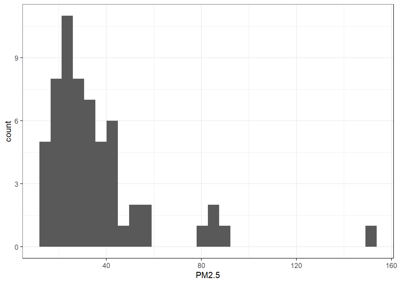
First I want to plot a histogram to check if the PM2.5 data follow a normal distribution (it should not)

ggplot(wff_data, aes(x= PM2.5))+
  geom_histogram()+
  theme_bw()

`stat_bin()` using `bins = 30`. Pick better value with `binwidth`.

The histogram confirms that the concentrations do not follow a normal distribution, since the data is right-skewed. This should follow a logarithmic distribution.

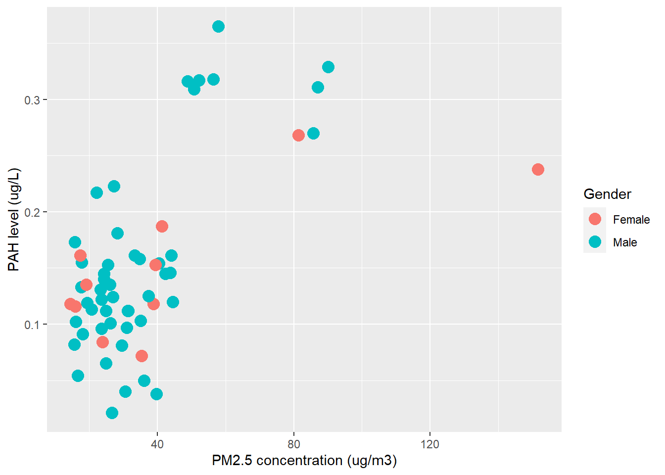
Here I am showing a plot to explore the association between the level of urine PAHs and PM2.5 concentration from the wildland firefighter subjects. I decided to separate them by gender.

ggplot(wff_data, aes(x= PM2.5, y= PAH, color= Gender))+
  geom_point(size= 4)+
  labs(x= "PM2.5 concentration (ug/m3)", y= "PAH level (ug/L)")

Based on the graphic, it seems that the level of PAHs is positively associated with PM2.5 concentration.

Next, I am showing a graph that explores the association between FVC and PM2.5.

ggplot(wff_data, aes(x= PM2.5, y=FVC))+
  geom_point(shape= 25, fill= "steelblue1", size= 3)+
  labs(x= "PM2.5 Concentration (ug/m3)", y= "FVC (L)")

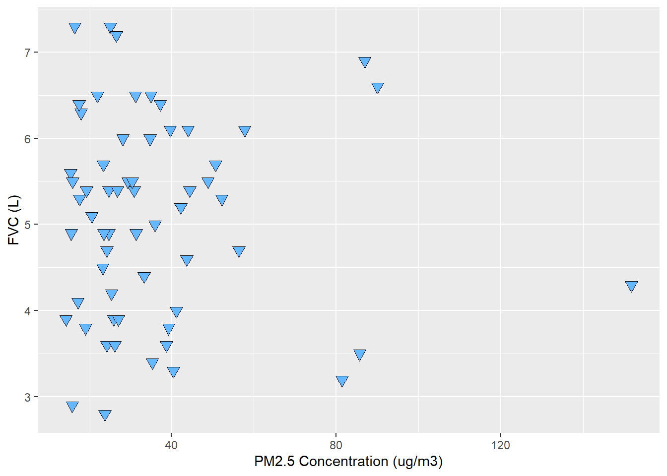
Based on this graph, it is hard to tell if FVC depends on PM2.5 concentration. Given so, I decided to fit a model and check for associations. In this case, since PM2.5 follows a log-normal distribution, I decided to use a log generalized linear model from the quasipoisson family. I used PM2.5, Smoking and Medication as predictors for FVC as an outcome.

log_fit <- glm(FVC ~ PM2.5 + Smoking + Medication, data = wff_data, family = quasipoisson(link = "log"))

summary(log_fit)


Call:
glm(formula = FVC ~ PM2.5 + Smoking + Medication, family = quasipoisson(link = "log"), 
    data = wff_data)

Coefficients:
              Estimate Std. Error t value Pr(>|t|)    
(Intercept)  1.6225347  0.0583858  27.790   <2e-16 ***
PM2.5       -0.0003841  0.0013235  -0.290    0.773    
Smoking      0.0238213  0.0883566   0.270    0.788    
Medication   0.0471521  0.0690668   0.683    0.498    
---
Signif. codes:  0 '***' 0.001 '**' 0.01 '*' 0.05 '.' 0.1 ' ' 1

(Dispersion parameter for quasipoisson family taken to be 0.2747653)

    Null deviance: 15.940  on 59  degrees of freedom
Residual deviance: 15.764  on 56  degrees of freedom
AIC: NA

Number of Fisher Scoring iterations: 4

Based on the log_fit model, it seems that there is no interaction of PM2.5 or any of the covariates to the FVC outcome. Which makes sense, since this outcome was mapped independently from the PM2.5 concentrations. However, in the real-life study I hope to find an association among these variables.

And finally, a model to explore if PM2.5 is a predictor of PAH levels. Also assessing Smoking and Medication as confounders.

log_fit2 <- glm(PAH ~ PM2.5 + Smoking + Medication, data = wff_data, family = quasipoisson(link = "log"))

summary(log_fit2)


Call:
glm(formula = PAH ~ PM2.5 + Smoking + Medication, family = quasipoisson(link = "log"), 
    data = wff_data)

Coefficients:
             Estimate Std. Error t value Pr(>|t|)    
(Intercept) -2.324968   0.100237 -23.195  < 2e-16 ***
PM2.5        0.009844   0.001714   5.743 3.96e-07 ***
Smoking      0.217576   0.144650   1.504    0.138    
Medication   0.081541   0.122211   0.667    0.507    
---
Signif. codes:  0 '***' 0.001 '**' 0.01 '*' 0.05 '.' 0.1 ' ' 1

(Dispersion parameter for quasipoisson family taken to be 0.02641762)

    Null deviance: 2.3605  on 59  degrees of freedom
Residual deviance: 1.5498  on 56  degrees of freedom
AIC: NA

Number of Fisher Scoring iterations: 5

In this case, we reject the null hypothesis that there is no association between PM2.5 and PAH levels (the outcome). Of course this was expected, since this was one of the requirements when creating the data set. Based on this model we didn’t find an association between smoking and the use of medication with the PAH outcome.