library(here)
library(readr)
library(tidyverse)
library(tidymodels)
library(gtsummary)
library(GGally)Fitting exercise
Mavoglurant modeling Exercise (Week 8)
These are the packages I used for this exercise
Loading the dataset, assigned it to the mavoglurant dataframe.
mavoglurant <- read_csv(here("fitting-exercise", "Mavoglurant_A2121_nmpk.csv"))Rows: 2678 Columns: 17
── Column specification ────────────────────────────────────────────────────────
Delimiter: ","
dbl (17): ID, CMT, EVID, EVI2, MDV, DV, LNDV, AMT, TIME, DOSE, OCC, RATE, AG...
ℹ Use `spec()` to retrieve the full column specification for this data.
ℹ Specify the column types or set `show_col_types = FALSE` to quiet this message.Data Cleaning
First, I created a plot showing the concentration of Mavoglurant DV over TIME, by DOSE. In the first attempt, the dose was plotted as a numeric variable so I mutated DOSE to be a categorical variable.
#Make `DOSE` a categorical variable using as.factor().
mavoglurant <- mavoglurant %>%
  mutate(DOSE = as.factor(DOSE))

#Create the plot of concentration by time, categorized by dose using ggplot().
ggplot(mavoglurant, aes(x = TIME, y = DV, group= ID)) +
  geom_line() + #Do a line plot
  facet_wrap(~ DOSE) + #Group by DOSE
  labs(x = "Time", y = "Mavoglurant concentration", color = "Dose")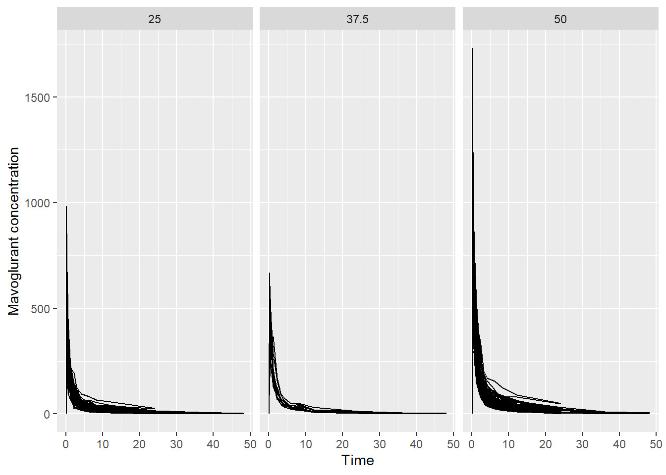
Now, keeping just one of the observations for individuals that have two OCC observations.
mavoglurant <- mavoglurant %>% filter(OCC == 1)Now, removing observations where TIME is equal to 0 and create a new dataframe mavoglurant_sum where it summarizes the concentrations from DV by each subject. Then, I created the mavoglurant_zero dataframe that contains only the observations where TIME is equal to 0. An finally I joined both new dataframes into the mavoglurant_new df.
# Exclude observations where 'TIME' = 0 and then compute the sum of 'DV' for each subject or 'ID', to create the `mavoglurant_sum` dataframe.
mavoglurant_sum <- mavoglurant %>%
  filter(TIME != 0) %>% #Remove observations where time= 0
  group_by(ID) %>% #Group by subject
  summarize(Y = sum(DV)) #The sum variable is called `Y`

#Create a dataframe with observations where TIME= 0.
mavoglurant_zero <- mavoglurant %>%
  filter(TIME == 0) %>%
  group_by(ID)

#Join the previous dataframes using left_join()
mavoglurant_new <- inner_join(mavoglurant_sum, mavoglurant_zero, by = "ID")
Finally, I filtered out unnecessary variables for this exercise and RACE, and SEX were converted to factor type variables.
#Mutate SEX and RACE to factory type variables and then only keep Y, DOSE, AGE, SEX, RACE, WT and HT.
mavoglurant_new <- mavoglurant_new %>%
  mutate(RACE = as.factor(RACE), SEX = as.factor(SEX)) %>%
  select(c(Y, DOSE, AGE, SEX, RACE, WT, HT))

#Check the structure of the new dataframe
str(mavoglurant_new)
tibble [120 × 7] (S3: tbl_df/tbl/data.frame)
$ Y : num [1:120] 2691 2639 2150 1789 3126 ...
$ DOSE: Factor w/ 3 levels "25","37.5","50": 1 1 1 1 1 1 1 1 1 1 ...
$ AGE : num [1:120] 42 24 31 46 41 27 23 20 23 28 ...
$ SEX : Factor w/ 2 levels "1","2": 1 1 1 2 2 1 1 1 1 1 ...
$ RACE: Factor w/ 4 levels "1","2","7","88": 2 2 1 1 2 2 1 4 2 1 ...
$ WT : num [1:120] 94.3 80.4 71.8 77.4 64.3 ...
$ HT : num [1:120] 1.77 1.76 1.81 1.65 1.56 ...#Save the cleaned dataframe as an .RDS file
write_rds(mavoglurant_new, here("ml-models-exercise", "mavoglurant.RDS"))Exploratory Data Analysis
The following plots and tables summarize the data observed from the mavoglurant_new dataframe.
First, a Boxplot that shows the dependent variable (Y) across the three different doses.
#Using ggplot() to create a boxplot of the predicted variable Y and the DOSE
ggplot(mavoglurant_new, aes(x= DOSE, y= Y))+
  geom_boxplot(fill= "aquamarine3")+
  theme_classic()+
  labs(x= "Dose", y= "Mavoglurant concentration")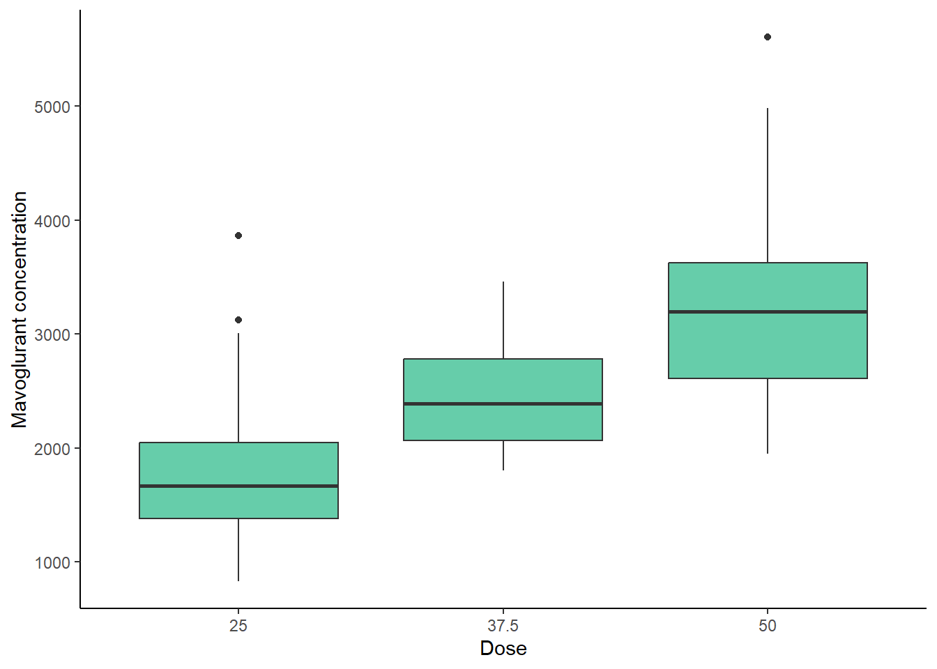
Based on the previous plot, it can be observed that at higher dose, the concentration of mavoglurant (predicted variable) increases. It is also seen that the range of concentrations is higher at the higher dose (50).
Now some plots that show the distribution of the dependent variable (Y) and the numeric independent variables AGE, WT and HT.
#Histogram of the dependent variable (Y)
ggplot(mavoglurant_new, aes(x= Y))+
  geom_histogram(fill= "aquamarine3", color= "red")+
  labs(x= "Mavoglurant concentration")
`stat_bin()` using `bins = 30`. Pick better value with `binwidth`.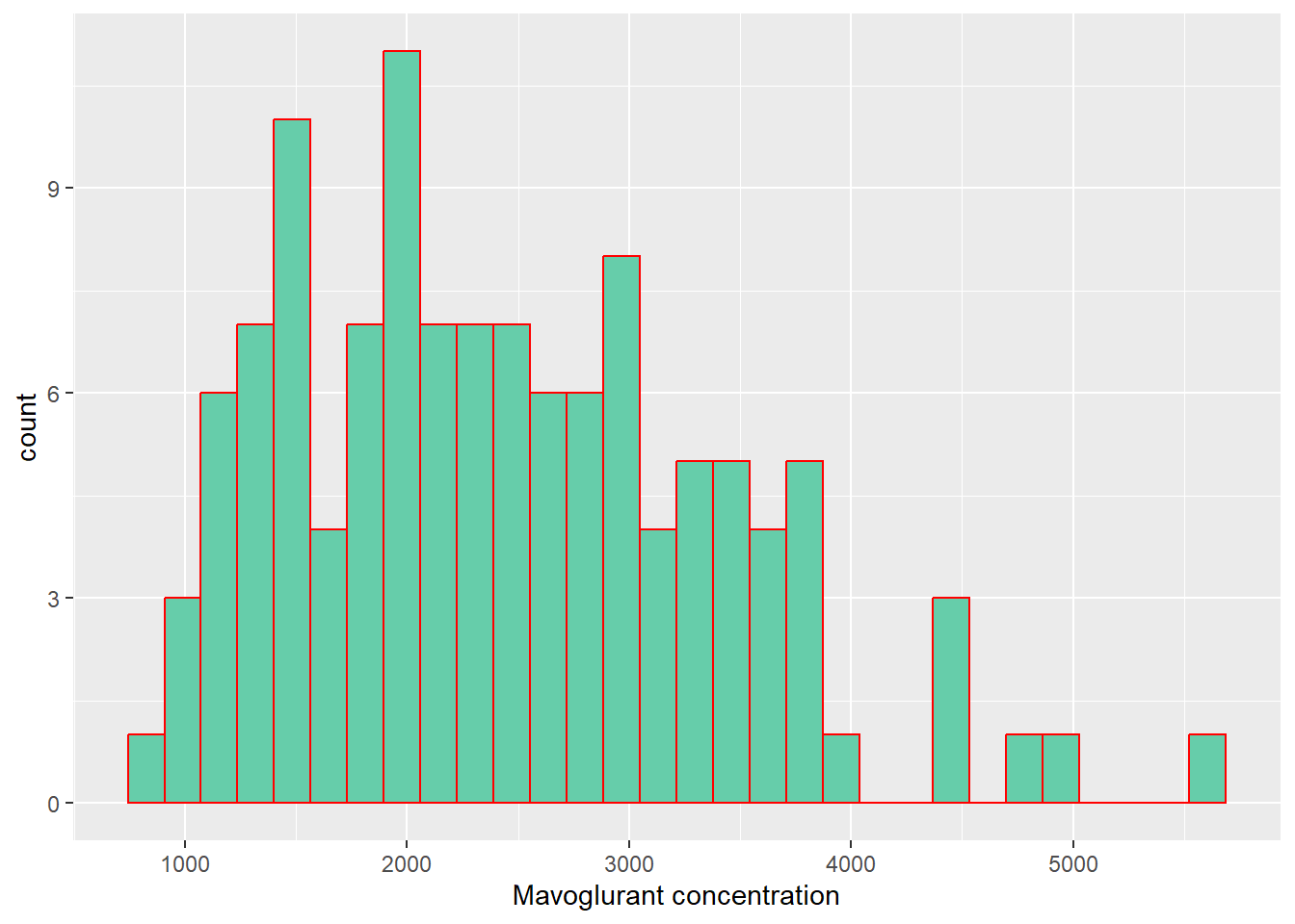
#Histogram of AGE
ggplot(mavoglurant_new, aes(x= AGE))+
  geom_histogram(fill= "darkgoldenrod1", color= "red")+
  labs(x= "Age")
`stat_bin()` using `bins = 30`. Pick better value with `binwidth`.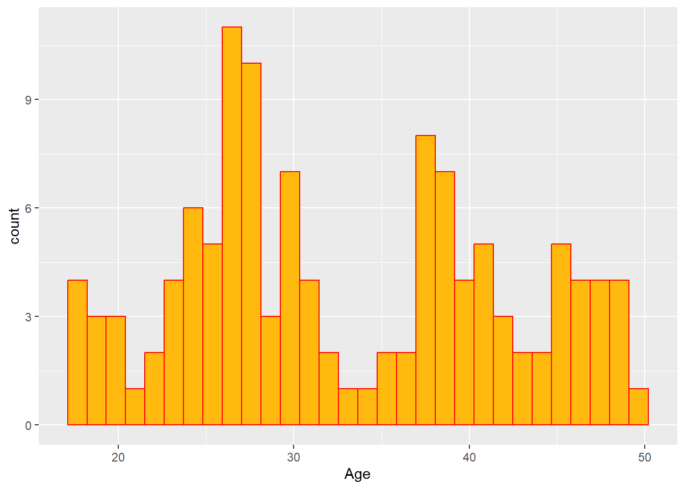
#Histogram of WT
ggplot(mavoglurant_new, aes(x= WT))+
  geom_histogram(fill= "darkgoldenrod1", color= "red")+
  labs(x= "Weight")
`stat_bin()` using `bins = 30`. Pick better value with `binwidth`.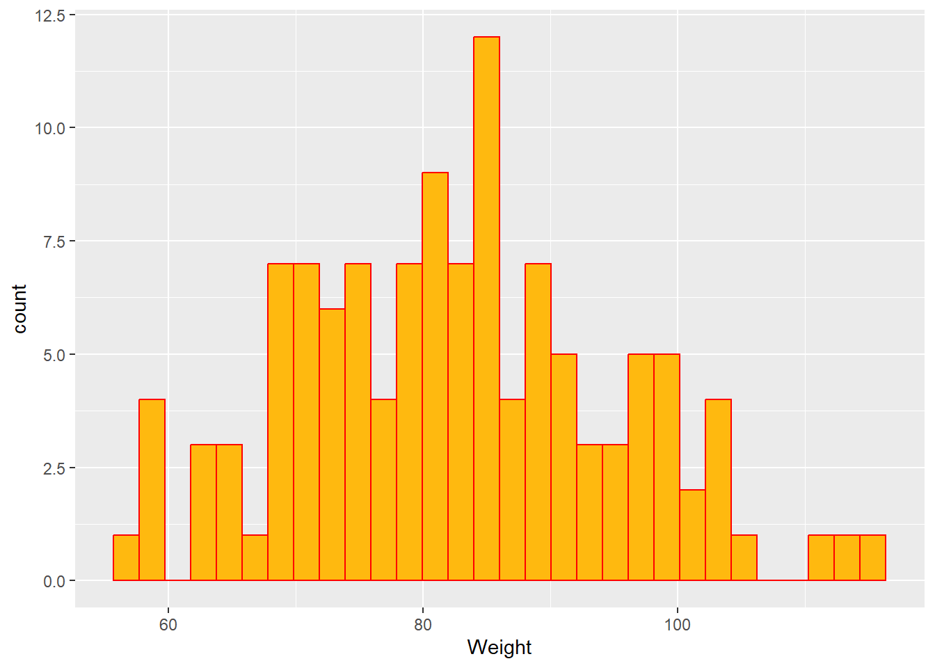
#Histogram of HT
ggplot(mavoglurant_new, aes(x= HT))+
  geom_histogram(fill= "darkgoldenrod1", color= "red")+
  labs(x= "Height")
`stat_bin()` using `bins = 30`. Pick better value with `binwidth`.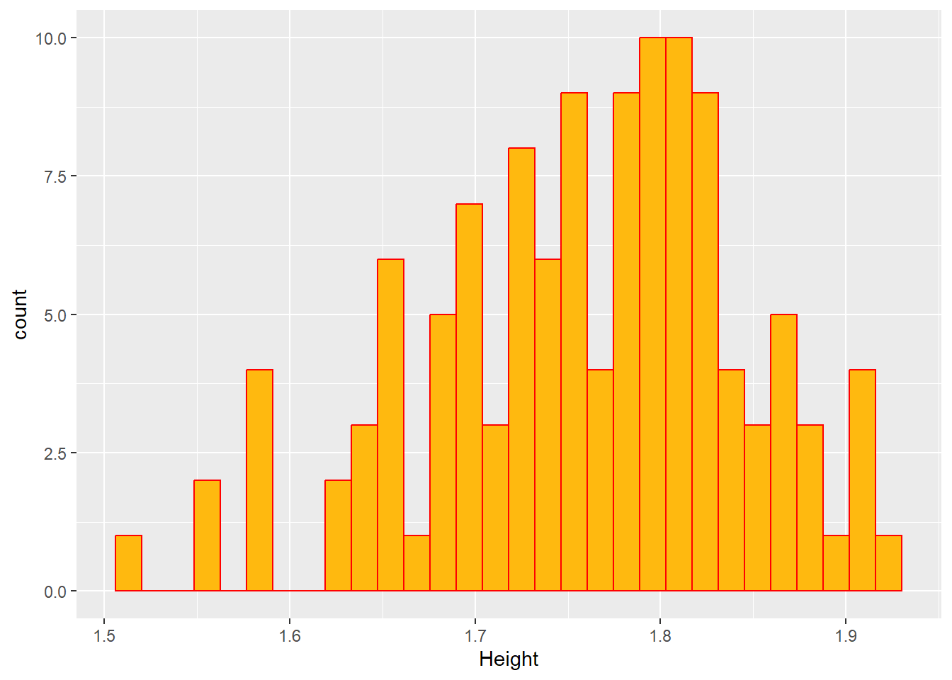
In the previous plots in can be seen that the dependent (Y) variable and the Weight, follow a normal distribution. Height is observed that is skewed to the right, so this variable could not be following a normal distribution. On the other hand, it is observed that Age follows a bi-modal distribution. This is providing an insight about maybe first applying a regression model to this dataset.
The following table summarizes the previous variables, categorized by SEX (1 or 2). Here, it is shown the mean (sd), median (IQR) and the range.
#Creating a summary table using the tbl_summary() function from `gtsummary`
sumtable <- mavoglurant_new %>% select(Y, AGE, HT, WT, SEX) %>%
  tbl_summary(by= SEX,
              type = all_continuous() ~ "continuous2",
              statistic = all_continuous() ~ c("{mean} ({sd})", "{median} ({p25}, {p75})", "{min}, {max}")) %>%
  bold_labels()

#Visualize the table
sumtable| Characteristic | 1, N = 104 | 2, N = 16 |
|---|---|---|
| Y | ||
| Mean (SD) | 2,478 (959) | 2,236 (983) |
| Median (IQR) | 2,398 (1,727, 3,072) | 2,060 (1,491, 2,698) |
| Range | 826, 5,607 | 1,044, 4,835 |
| AGE | ||
| Mean (SD) | 32 (9) | 41 (7) |
| Median (IQR) | 30 (25, 39) | 42 (38, 45) |
| Range | 18, 49 | 28, 50 |
| HT | ||
| Mean (SD) | 1.78 (0.07) | 1.63 (0.06) |
| Median (IQR) | 1.78 (1.73, 1.82) | 1.63 (1.58, 1.66) |
| Range | 1.59, 1.93 | 1.52, 1.75 |
| WT | ||
| Mean (SD) | 84 (12) | 73 (11) |
| Median (IQR) | 83 (75, 92) | 70 (64, 81) |
| Range | 57, 115 | 58, 90 |
And here, showing barplots for the categorical variables SEX and RACE.
#Creating a bar plot that shows the counts for each race category by sex.
ggplot(mavoglurant_new, aes(x= RACE, fill= SEX))+
  geom_bar(position = "dodge")+
  theme_classic()+
  labs(x= "Race")
It is observed on the previous plot that there are more subjects of sex 1, than 2 for the 1, 2 and 88 race categories. Meanwhile for the race category 7, it seems that there is the same amount of subjects by sex category. It is a shame that the correct labels for these categories are not known for sure.
And finally, exploring correlations between all the variables, visualizing by a plot:
#Creating a correlation plot using the ggpairs() function from the GGally package.
ggpairs(mavoglurant_new, columns = c(1, 3, 6, 7), progress = F)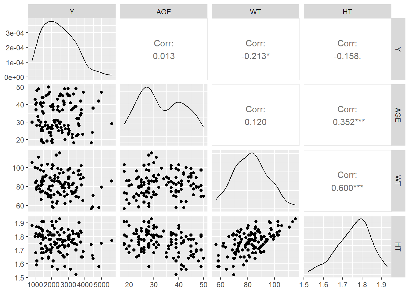
Based on this plot it is observed that the highest correlation is between the variables Height and Weight (0.6), and the linear plots in the middle confirm the distribution of each one of the variables.
Model Fitting
Linear Regression Models
First, I fitted a linear model using the continuous outcome (Y) and DOSE as the predictor.
# Define the model specification for linear regression
linear_model <- linear_reg() %>%
  set_engine("lm") %>% #Specify the linear model to fit the model
  set_mode("regression") #Setting the mode as a regression model

# Define the formula
formula1 <- Y ~ DOSE

# Fit the model
lm_simple <- linear_model %>%
  fit(formula1, data = mavoglurant_new) #Calling the formula and the dataframe to compute the linear model

# Output the model summary
summary(lm_simple$fit)
Call:
stats::lm(formula = Y ~ DOSE, data = data)

Residuals:
    Min      1Q  Median      3Q     Max
-1290.1  -445.6   -90.9   352.2  2367.7

Coefficients:
            Estimate Std. Error t value Pr(>|t|)
(Intercept)  1782.67      87.85  20.292  < 2e-16 ***
DOSE37.5      681.24     213.69   3.188  0.00184 **
DOSE50       1456.20     130.43  11.165  < 2e-16 ***
---
Signif. codes:  0 '***' 0.001 '**' 0.01 '*' 0.05 '.' 0.1 ' ' 1

Residual standard error: 674.8 on 117 degrees of freedom
Multiple R-squared:  0.5159,    Adjusted R-squared:  0.5076
F-statistic: 62.33 on 2 and 117 DF,  p-value: < 2.2e-16
Based on the model it can be inferred that the outcome increases by around 681.24 units with the dose 37.5 and increases by 1456.20 with the dose 50, all compared with the dose 25. It is also observed that the differences are statistically significant, given the p-values are less than 0.001.
Now, fitting a linear model using the continuous outcome (Y) and using the rest of the variables as predictors.
#The model specification has already been set in the previous code chunk, so there is no need to set it again.

# Define the formula
formula2 <- Y ~ AGE + WT + HT + DOSE + SEX + RACE

# Fit the model
lm_multi <- linear_model %>%
  fit(formula2, data = mavoglurant_new)

# Output the model summary
summary(lm_multi$fit)
Call:
stats::lm(formula = Y ~ AGE + WT + HT + DOSE + SEX + RACE, data = data)

Residuals:
     Min       1Q   Median       3Q      Max
-1496.97  -362.81   -71.26   285.84  2421.48

Coefficients:
            Estimate Std. Error t value Pr(>|t|)
(Intercept) 4890.923   1822.710   2.683 0.008415 **
AGE            3.521      7.895   0.446 0.656517
WT           -23.281      6.440  -3.615 0.000454 ***
HT          -741.050   1108.100  -0.669 0.505051
DOSE37.5     663.683    200.448   3.311 0.001258 **
DOSE50      1499.048    122.462  12.241  < 2e-16 ***
SEX2        -360.048    217.775  -1.653 0.101121
RACE2        148.883    129.821   1.147 0.253936
RACE7       -420.950    451.163  -0.933 0.352846
RACE88       -65.300    246.961  -0.264 0.791954
---
Signif. codes:  0 '***' 0.001 '**' 0.01 '*' 0.05 '.' 0.1 ' ' 1

Residual standard error: 616.6 on 110 degrees of freedom
Multiple R-squared:   0.62, Adjusted R-squared:  0.5889
F-statistic: 19.94 on 9 and 110 DF,  p-value: < 2.2e-16
For the interpretation of this model I will focus only on the statistically significant predictors (p-value < 0.001). Besides dose 37.5 with an increase of the outcome by a factor of ~664 and dose 50 with an increase by a factor of ~1500, Weight is also another variable associated with a decrease of the outcome by a factor of ~23.
In summary, it can be observed that the coefficients slightly changed between both models, however the second model seems a better fit. To evaluate which model is best, I computed the root mean square error (RMSE) and R-squared as metrics. First for the linear model using one predictor, and then using multiple predictors.
#ONE VARIABLE AS PREDICTOR
#Create a prediction from the dataframe
lmsimple_pred <- predict(lm_simple, new_data = mavoglurant_new %>% select(-Y))

#Match predicted with observed
lmsimple_pred <- bind_cols(lmsimple_pred, mavoglurant_new %>% select(Y))

#Estimate the metrics
lmsimple_metrics <- metric_set(rmse, rsq)
lmsimple_metrics(lmsimple_pred, truth = Y, estimate = .pred)
# A tibble: 2 × 3
.metric .estimator .estimate
<chr> <chr> <dbl>
1 rmse standard 666.
2 rsq standard 0.516#MULTIPLE VARIABLES AS PREDICTORS
#Create a prediction from the dataframe
lmmulti_pred <- predict(lm_multi, new_data = mavoglurant_new %>% select(-Y))
#Match predicted with observed
lmmulti_pred <- bind_cols(lmmulti_pred, mavoglurant_new %>% select(Y))
#Estimate the metrics
lmmulti_metrics <- metric_set(rmse, rsq)
lmmulti_metrics(lmmulti_pred, truth = Y, estimate = .pred)# A tibble: 2 × 3
.metric .estimator .estimate
<chr> <chr> <dbl>
1 rmse standard 590.
2 rsq standard 0.620We can observe that the RMSE is lower (590.3) in the model that inputs all the variables as predictors compared to the linear model that uses Dose as a predictor (RMSE= 666.3). We also observe that the R2 is slightly higher in the second model (0.62) compared to the first model (0.52). In this case we can conclude that the second model (linear model with multiple predictors) is a better fit to this dataset.
Logistic Models
Now, I fitted a logistic model to the outcome SEX, and using DOSE as a predictor. I also evaluated the Accuracy and ROC-AUC of this model in the following steps.
# Define the model specification
logistic_spec <- logistic_reg() %>%  #Defining as logistic
  set_engine("glm") %>% #...From the GLM family
  set_mode("classification") #Classification, since it involves categorical variables

# Create the recipe
recipe <- recipe(SEX ~ DOSE, data = mavoglurant_new) %>%
  step_dummy(all_nominal(), -all_outcomes())

# Split the data into training and testing sets
set.seed(123) #For reproducibility
data_split <- initial_split(mavoglurant_new, prop = 0.75)
train_data <- training(data_split) #Create a training data to apply the model
test_data <- testing(data_split) #Create a test data to apply the model evaluation

# Fit the model
logistic_fit <- workflow() %>%
  add_recipe(recipe) %>%
  add_model(logistic_spec) %>%
  fit(data = train_data)

# Make predictions on the test set to determine the ROC-AUC of the model
predictions <- predict(logistic_fit, test_data, type = "prob")

#Make predictions on the test set to determine the Accuracy of the model
predictions2 <- logistic_fit %>% predict(new_data = test_data)

# Bind the predictions to the testing set
results <- bind_cols(test_data, predictions) #ROC-AUC
results2 <- bind_cols(test_data, predictions2) #Accuracy

# Calculate ROC-AUC
roc_auc <- roc_auc(results, truth = SEX, .pred_1)

# Calculate Accuracy
accuracy <- accuracy(results2, truth = SEX, estimate = .pred_class)

# Output the model and the metrics
log1 <- glm(formula = SEX ~ DOSE, family = binomial(link = "logit"),
    data = train_data)
summary(log1)
Call:
glm(formula = SEX ~ DOSE, family = binomial(link = "logit"),
    data = train_data)

Coefficients:
            Estimate Std. Error z value Pr(>|z|)
(Intercept)  -1.3581     0.3737  -3.634 0.000279 ***
DOSE37.5      0.2595     0.8980   0.289 0.772583
DOSE50       -1.0986     0.7082  -1.551 0.120851
---
Signif. codes:  0 '***' 0.001 '**' 0.01 '*' 0.05 '.' 0.1 ' ' 1

(Dispersion parameter for binomial family taken to be 1)

    Null deviance: 77.801  on 89  degrees of freedom
Residual deviance: 74.572  on 87  degrees of freedom
AIC: 80.572

Number of Fisher Scoring iterations: 5list(Accuracy = accuracy, ROC_AUC = roc_auc)$Accuracy
# A tibble: 1 × 3
.metric .estimator .estimate
<chr> <chr> <dbl>
1 accuracy binary 0.933
$ROC_AUC
# A tibble: 1 × 3
.metric .estimator .estimate
<chr> <chr> <dbl>
1 roc_auc binary 0.393And finally, fitting a logistic model to the outcome SEX, using all of the variables as predictors. I also computed the ROC-AUC and Accuracy of this model.
# The model has been defined before 'logistic_spec', so there is no need to define it again.

# Create the recipe of this model
recipe2 <- recipe(SEX ~ Y + AGE + WT + HT + DOSE + RACE, data = mavoglurant_new) %>%
  step_dummy(all_nominal(), -all_outcomes()) %>%
  step_zv(all_predictors()) %>%
  step_normalize(all_predictors())

# Split the data into training and testing sets
set.seed(123) #For reproducibility
data_split2 <- initial_split(mavoglurant_new, prop = 0.75)
train_data2 <- training(data_split2) #Create a training data to apply the model
test_data2 <- testing(data_split2) #Create a test data to apply the model evaluation

# Fit the model
logistic_fit2 <- workflow() %>%
  add_recipe(recipe2) %>%
  add_model(logistic_spec) %>%
  fit(data = train_data)
Warning: glm.fit: fitted probabilities numerically 0 or 1 occurred# Make predictions on the test set to determine the ROC-AUC of the model
predictions_auc <- predict(logistic_fit2, test_data2, type = "prob")
#Make predictions on the test set to determine the Accuracy of the model
predictions_acc <- logistic_fit %>% predict(new_data = test_data2)
# Bind the predictions to the testing set
results_auc2 <- bind_cols(test_data2, predictions_auc) #ROC-AUC
results_acc2 <- bind_cols(test_data2, predictions_acc) #Accuracy
# Calculate ROC-AUC
roc_auc2 <- roc_auc(results_auc2, truth = SEX, .pred_1)
# Calculate Accuracy
accuracy2 <- accuracy(results_acc2, truth = SEX, estimate = .pred_class)
# Output the metrics using list()
log2 <- glm(formula = SEX ~ Y + AGE + WT + HT + DOSE + RACE, family = binomial(link = "logit"),
data = train_data2)Warning: glm.fit: fitted probabilities numerically 0 or 1 occurredsummary(log2)
Call:
glm(formula = SEX ~ Y + AGE + WT + HT + DOSE + RACE, family = binomial(link = "logit"),
    data = train_data2)

Coefficients:
              Estimate Std. Error z value Pr(>|z|)
(Intercept) 119.467600  47.800737   2.499   0.0124 *
Y            -0.002105   0.002031  -1.036   0.3000
AGE           0.319506   0.174943   1.826   0.0678 .
WT           -0.190608   0.130000  -1.466   0.1426
HT          -64.948813  26.352756  -2.465   0.0137 *
DOSE37.5     -7.347424   8.122569  -0.905   0.3657
DOSE50       -3.665713   5.095677  -0.719   0.4719
RACE2        -6.722388   4.881126  -1.377   0.1684
RACE7        -3.259653  17.820091  -0.183   0.8549
RACE88       -5.593682  12.167640  -0.460   0.6457
---
Signif. codes:  0 '***' 0.001 '**' 0.01 '*' 0.05 '.' 0.1 ' ' 1

(Dispersion parameter for binomial family taken to be 1)

    Null deviance: 77.801  on 89  degrees of freedom
Residual deviance: 12.013  on 80  degrees of freedom
AIC: 32.013

Number of Fisher Scoring iterations: 10list(Accuracy = accuracy2, ROC_AUC = roc_auc2)$Accuracy
# A tibble: 1 × 3
.metric .estimator .estimate
<chr> <chr> <dbl>
1 accuracy binary 0.933
$ROC_AUC
# A tibble: 1 × 3
.metric .estimator .estimate
<chr> <chr> <dbl>
1 roc_auc binary 0.964Based on the previous logistic models, it is observed that appears there is no association between the dose of mavoglurant and sex. However, when observing the second logistic model, it appears there is a statistically significant association between height and sex (p-value < 0.05). While looking at the accuracy from both models, we can see that both have the same accuracy (93%), however, the ROC-AUC value is pretty low for the model that uses only Dose as a predictor (0.39), meanwhile, the model that uses dose and all the other variables as predictors has a better value (0.96), which reflects better sensitivity and specificity.
Mavoglurant modeling Exercise continuation (Week 10)
First, naming the seed for reproducibility
rngseed = 1234
set.seed(rngseed)
Remove the RACE variable from the mavoglurant_new dataframe.
#Select all other variables, except `RACE`
mavoglurant_new <- mavoglurant_new %>% select(-RACE)
Split the data randomly to a 75% train and 25% test data.
#Let the data split be 75-25% or 3/4
data_split3 <- initial_split(mavoglurant_new, prop = 0.75)

#Create the train and test data frames
train_data3 <- training(data_split3)
test_data3 <- testing(data_split3)
Model performance assessment 1
Now, fitting a linear regression model that predicts the outcome Y based on DOSE alone. Then, making predictions to compare against the observed values and then computing the RMSE to evaluate.
#Define the model specification for linear regression
lm_dose <- linear_reg() %>%
  set_engine("lm") %>% #Specify the linear model to fit the model
  set_mode("regression") %>% #Setting the mode as a regression model
  fit(Y ~ DOSE, data = train_data3)

#Tidy the results
tidy(lm_dose)
# A tibble: 3 × 5
term estimate std.error statistic p.value
<chr> <dbl> <dbl> <dbl> <dbl>
1 (Intercept) 1873. 109. 17.2 1.07e-29
2 DOSE37.5 651. 275. 2.36 2.03e- 2
3 DOSE50 1336. 158. 8.45 5.97e-13#Create a prediction from the dataframe for the `DOSE` model
lmdose_pred <- predict(lm_dose, new_data = train_data3)
#Match predicted with observed values
lmdose_pred <- bind_cols(lmdose_pred, train_data3)
#Estimate the metrics for the `DOSE` model
lmdose_metric <- metric_set(rmse) #Set the function to estimate RMSE
lmdose_metric(lmdose_pred, truth = Y, estimate = .pred) #Compute the RMSE# A tibble: 1 × 3
.metric .estimator .estimate
<chr> <chr> <dbl>
1 rmse standard 703.Computing another linear regression model that predicts Y using the other variables as predictors. I also computed the predicted vs observed values to compute the RMSE of this model.
#Define the model specification for linear regression
lm_all <- linear_reg() %>%
  set_engine("lm") %>% #Specify the linear model to fit the model
  set_mode("regression") %>% #Setting the mode as a regression model
  fit(Y ~ ., data = train_data3)

#Tidy the results
tidy(lm_all)
# A tibble: 7 × 5
term estimate std.error statistic p.value
<chr> <dbl> <dbl> <dbl> <dbl>
1 (Intercept) 5764. 2178. 2.65 9.72e- 3
2 DOSE37.5 640. 255. 2.51 1.39e- 2
3 DOSE50 1384. 147. 9.44 8.65e-15
4 AGE -0.119 9.66 -0.0123 9.90e- 1
5 SEX2 -571. 287. -1.99 5.00e- 2
6 WT -22.8 7.72 -2.95 4.13e- 3
7 HT -1117. 1368. -0.817 4.17e- 1#Create a prediction from the dataframe of the model with all the other predictors
lmall_pred <- predict(lm_all, new_data = train_data3)
#Match predicted with observed
lmall_pred <- bind_cols(lmall_pred, train_data3)
#Estimate the metrics for the model with all the variables as predictors
lmall_metric <- metric_set(rmse) #Set the function
lmall_metric(lmall_pred, truth = Y, estimate = .pred) #Compute the RMSE# A tibble: 1 × 3
.metric .estimator .estimate
<chr> <chr> <dbl>
1 rmse standard 627.Now I created a null model and computed the RMSE.
#Run the null model
lm_null <- null_model(mode = "regression") %>%
    set_engine("parsnip") %>%
    fit(Y ~ 1, data = train_data3)

#Compute the RMSE and other estimates
null_metric <- lm_null %>%
  predict(train_data3) %>%
  bind_cols(train_data3) %>%
  metrics(truth = Y, estimate = .pred)
Warning: A correlation computation is required, but `estimate` is constant and has 0
standard deviation, resulting in a divide by 0 error. `NA` will be returned.#Print the RMSE (Note: This includes also the R-squared and MAE but I am only interested in the RMSE)
null_metric# A tibble: 3 × 3
.metric .estimator .estimate
<chr> <chr> <dbl>
1 rmse standard 948.
2 rsq standard NA
3 mae standard 765.In summary, according to the RMSE parameters, the model that includes all the variables as predictors performed better (RMSE= 627), compared to the model using only DOSE as a predictor (RMSE= 702) and the null model (RMSE= 948) as a reference.
Model performance assessment 2
Now, evaluating both models using a 10-fold cross-validation. First, by the model that predicts Y only using DOSE.
#Set the seed for reproducibility
set.seed(rngseed)

#Set the cross-validation folds as 10
folds <- vfold_cv(train_data3, v= 10)

#Set the model specification, for linear regression
linear_mod <- linear_reg() %>% set_engine("lm")

#Set the workflow
linear_wf <- workflow() %>% add_model(linear_mod) %>% add_formula(Y ~ DOSE)

#Do the resamples
dose_resample <- fit_resamples(linear_wf, resamples = folds)

#Extract the metric
collect_metrics(dose_resample)
# A tibble: 2 × 6
.metric .estimator mean n std_err .config
<chr> <chr> <dbl> <int> <dbl> <chr>
1 rmse standard 697. 10 68.1 Preprocessor1_Model1
2 rsq standard 0.500 10 0.0605 Preprocessor1_Model1Now, doing the cross-validation for the model that predicts Y using all the other variables as predictors.
#Set the seed for reproducibility
set.seed(rngseed)

#Set the workflow
linear_all_wf <- workflow() %>% add_model(linear_mod) %>% add_formula(Y ~ .)

#Do the resamples
all_resample <- fit_resamples(linear_all_wf, resamples = folds)

#Extract the metric
collect_metrics(all_resample)
# A tibble: 2 × 6
.metric .estimator mean n std_err .config
<chr> <chr> <dbl> <int> <dbl> <chr>
1 rmse standard 653. 10 63.6 Preprocessor1_Model1
2 rsq standard 0.561 10 0.0717 Preprocessor1_Model1Based on the previous results, it can be observed that when fitting the model and conducting a 10-fold cross-validation the RMSEs changed but still, the model that uses all predictors have a better metric (RMSE= 653, SE= 63.6) than the model that uses only DOSE as a predictor (RMSE= 696, SE= 68).
And now, computing the same CV analysis, but setting a different seed.
#Set the seed for reproducibility
set.seed(2302)

#Set the cross-validation folds as 10
folds2 <- vfold_cv(train_data3, v= 10)

#Set the model specification, for linear regression
linear_mod2 <- linear_reg() %>% set_engine("lm")

#ONE PREDICTOR LINEAR MODEL
#Set the workflow
linear_wf2 <- workflow() %>% add_model(linear_mod2) %>% add_formula(Y ~ DOSE)

#Do the resamples
dose_resample2 <- fit_resamples(linear_wf2, resamples = folds2)

#Extract the metric
collect_metrics(dose_resample2)
# A tibble: 2 × 6
.metric .estimator mean n std_err .config
<chr> <chr> <dbl> <int> <dbl> <chr>
1 rmse standard 706. 10 53.3 Preprocessor1_Model1
2 rsq standard 0.451 10 0.0690 Preprocessor1_Model1#ALL PREDICTORS LINEAR MODEL
#Set the workflow
linear_all_wf2 <- workflow() %>% add_model(linear_mod2) %>% add_formula(Y ~ .)
#Do the resamples
all_resample2 <- fit_resamples(linear_all_wf2, resamples = folds2)
#Extract the metric
collect_metrics(all_resample2)# A tibble: 2 × 6
.metric .estimator mean n std_err .config
<chr> <chr> <dbl> <int> <dbl> <chr>
1 rmse standard 660. 10 57.5 Preprocessor1_Model1
2 rsq standard 0.516 10 0.0613 Preprocessor1_Model1In this case, when changing the seed, the metrics changed for both models but they are similar in proportion. For the linear model with a single predictor the RMSE= 705.9 and for the model with all predictors the RMSE= 660. However, the standar error is higher for the model with all the predictors (SE= 57.51), compared to the model with a single predictor (SE= 53.33). Still, it seems that the linear model that uses all the predictors is better than the model that uses only DOSE as a single predictor.
This section is added by Malika Dhakhwa.
I conducted a visual inspection of performance of the models by plotting the predicted values from all three models against the observed values of the training data.
First, I extracted the predicted values of the Null model.For the other two models, this step has already been completed in earlier phases.
# Recovering predicted values of the null model
null_pred <- predict(lm_null, new_data = train_data3)
I created a combined data frame of the predictors in long format for all three models and created the plot.
#Creating the object for the outcome variable Y in the training data
observed_values <- train_data3$Y

#Creating separate data frames for each set of predictions with model labels

df_dose <- data.frame(Observed = observed_values, Predicted = lmdose_pred$.pred, Model="Dose Model")
df_all <- data.frame(Observed= observed_values, Predicted = lmall_pred$.pred, Model="Full Model")
df_null<- data.frame(Observed = observed_values, Predicted = null_pred$.pred, Model="Null Model")

#Combining all the predicted values to a single data frame by rows to create a long format data
combined_df <- rbind(df_dose, df_all, df_null)

#Plotting of predicted vs observed data
ggplot(combined_df, aes(x=Observed, y=Predicted, color=Model))+
  geom_point()+
  scale_color_manual(values = c("Null Model"= "lightblue", "Dose Model"="red", "Full Model"="green")) +
  geom_abline(intercept = 0, slope = 1, linetype = "solid", color="black") + #45 degree line
  xlim(0, 5000) + #X-axis limits
  ylim(0, 5000) + #y-axis limits
  labs(x= "Observed Values", y ="Predicted Values", title = "Predicted vs. Observed Values")+
  theme_minimal() # Use a minimal theme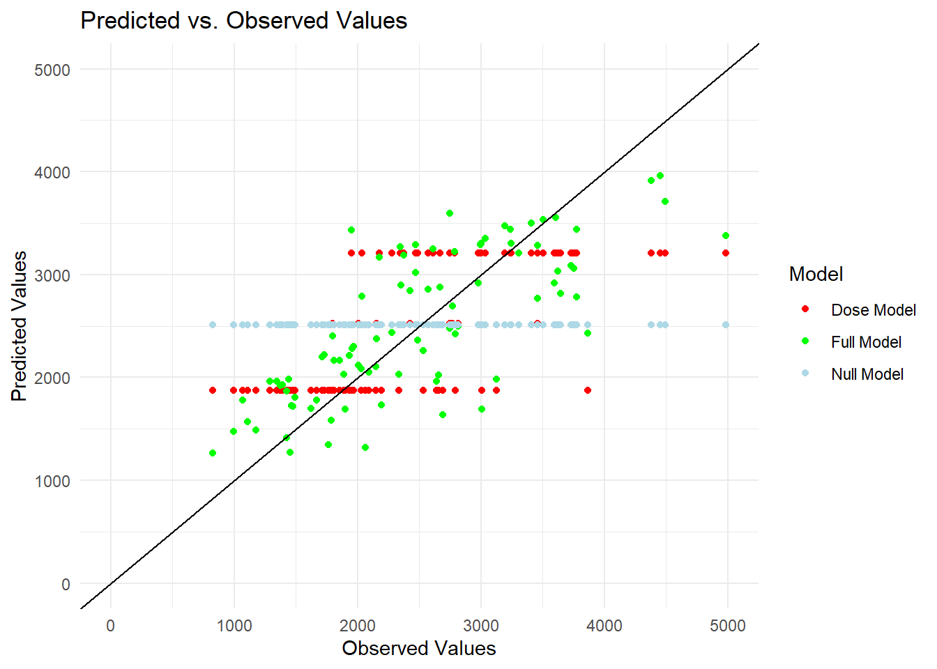
The predictions from Null model follows a horizontal line indicating that they assume a single value which is the mean of the outcome variable. The variable Dose in the observed data has only three distinct values, leading the Dose model’s predictions to appear as three horizontal lines in the plot, marked by red dots. One of these predicted values is close to that of the Null model, creating almost overlapping with the predictions from the Null model. The predicted values from the model incorporating all predictors are more dispersed indicating that this model is better than the other two models. However, the scatter still exhibits some pattern. To further investigate the existence of any patterns, I plotted the predicted values against the residuals for this comprehensive model.
First, I computed the residuals and subsequently generated the plot.
#creating an object for the full model from the combined data adding a column of Residuals
all_vars_residuals <- combined_df %>%
  filter(Model == "Full Model")%>%
  mutate(Residuals = Predicted - Observed)

# plotting Predicted vs. Residuals for the full model

ggplot(all_vars_residuals, aes(x = Predicted, y = Residuals)) +
  geom_point(color = "darkblue") + # Plot the residuals
  geom_hline(yintercept = 0, linetype = "solid", color = "darkred") + # Add a horizontal line at 0
  labs(x = "Predicted Values", y = "Residuals", title = "Residuals vs. Predicted Values (Full Model)") +
  ylim(-2500, 2500) +  #y-axis limits
  theme_minimal() # Use a minimal theme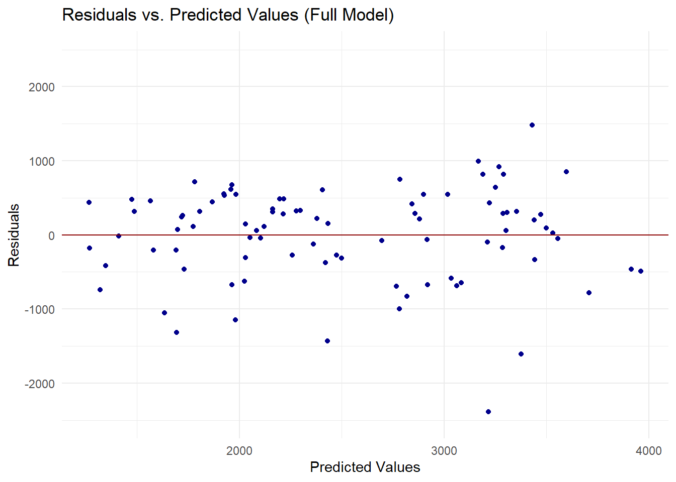
The residuals are not randomly scattered around the zero line. We can see that there is a discernible pattern suggesting that the model may not be capturing some of the data features.
Model Uncertainty Assessment with Bootstrap
I assessed the variability of the predicted values by employing bootstrap resampling, drawing 100 samples from the training data. For each sample, I refitted the comprehensive model that includes all the predictors. The goal is to measure the uncertainty present in the model’s predictions.
#Setting the seed same as at the beginning of the exercise for reproducibility
set.seed(rngseed)

#Creating 100 bootstrap samples from the training data
boot_samples <-bootstraps(train_data3, times = 100)

#Following codes help check any bootstrap sample if needed
dat_sample <- rsample::analysis(boot_samples$splits[[57]]) #Replace [[57]] by [[relevant sample no.from 1 to 100]] to view that sample
#dat_sample
I fitted the model to each Bootstrap sample and collected the predictions into a list using the map function.I converted the list to a matrix to simplify data manipulation.
# Setting the function to fit model and make predictions
fit_and_predict <- function(boot) {
  # Fit the model to the bootstrap sample
  lm_all_bs <- linear_reg() %>%
    set_engine("lm") %>%
    set_mode("regression") %>%
    fit(Y ~ ., data = analysis(boot))

  # Make predictions on the original training data
  predictions <- predict(lm_all_bs, new_data = train_data3)$.pred

  return(predictions)
}

# Applying the function to each bootstrap sample and collecting predictions
predictions_list <- map(boot_samples$splits, fit_and_predict)

# Converting the list of predictions to a matrix
predictions_matrix <- do.call(cbind, predictions_list)
I computed the means, medians and 89% confidence intervals of the predictions for each of the samples.
# Calculating the mean prediction for each sample
mean_predictions <- rowMeans(predictions_matrix)

#Computing median and 89% Confidence Interval
preds <-predictions_matrix %>%
  apply(1, quantile, c(0.055, 0.5, 0.945))%>%
  t()

#mean_predictions
preds
5.5% 50% 94.5%
[1,] 3095.536 3345.767 3553.229
[2,] 1688.124 1962.397 2185.772
[3,] 2420.566 2717.821 2937.470
[4,] 1798.039 2094.438 2386.281
[5,] 2660.761 2936.070 3141.177
[6,] 1066.095 1301.015 1490.740
[7,] 2176.857 2433.866 2661.169
[8,] 1699.532 1942.421 2292.867
[9,] 1290.691 1540.256 1879.126
[10,] 2271.149 2516.569 2752.715
[11,] 1295.460 1559.158 1886.120
[12,] 1730.178 1914.622 2143.851
[13,] 2002.008 2437.799 2755.797
[14,] 2935.489 3295.735 3623.611
[15,] 1757.794 2000.467 2240.672
[16,] 2043.776 2254.439 2480.689
[17,] 3168.574 3432.252 3730.375
[18,] 2615.269 2960.192 3268.438
[19,] 1966.970 2350.748 2850.072
[20,] 3071.362 3278.368 3507.790
[21,] 3667.221 3987.499 4259.103
[22,] 3003.822 3238.672 3510.319
[23,] 1001.757 1288.117 1555.024
[24,] 2248.555 2742.403 3177.462
[25,] 2954.560 3205.178 3395.522
[26,] 2793.860 3113.973 3311.245
[27,] 2073.601 2506.080 2823.173
[28,] 1328.110 1510.954 1685.221
[29,] 1588.768 1812.558 2025.079
[30,] 1636.373 2017.330 2345.360
[31,] 2587.672 2831.790 3028.960
[32,] 3377.058 3568.144 3832.479
[33,] 1797.321 2022.020 2210.438
[34,] 1151.598 1319.471 1562.546
[35,] 1873.889 2107.277 2333.929
[36,] 1560.185 1723.784 1970.624
[37,] 2894.356 3220.719 3457.213
[38,] 3346.501 3715.141 4046.741
[39,] 1951.650 2176.815 2413.828
[40,] 1410.545 1779.102 2067.531
[41,] 1806.414 1970.386 2137.388
[42,] 2042.688 2229.645 2407.115
[43,] 1654.071 1863.188 2089.427
[44,] 3708.077 3923.919 4247.251
[45,] 3092.981 3342.049 3601.919
[46,] 3074.294 3458.830 3791.452
[47,] 1830.768 2038.590 2260.294
[48,] 1996.170 2208.096 2431.201
[49,] 3244.506 3475.193 3738.398
[50,] 3235.159 3480.633 3749.818
[51,] 2235.910 2429.083 2631.497
[52,] 2613.417 2897.492 3137.076
[53,] 1874.792 2126.913 2362.522
[54,] 3354.259 3567.665 3834.856
[55,] 2083.492 2282.726 2489.073
[56,] 1540.146 1703.919 1869.360
[57,] 2593.562 2878.157 3121.766
[58,] 1708.720 2040.540 2396.428
[59,] 3041.401 3319.502 3537.824
[60,] 1795.475 1980.278 2171.579
[61,] 2903.656 3118.823 3325.790
[62,] 1638.444 1922.457 2249.845
[63,] 1133.853 1375.503 1585.288
[64,] 3212.848 3390.520 3597.378
[65,] 1458.885 1698.531 1954.253
[66,] 3006.204 3285.482 3523.127
[67,] 3006.686 3377.229 3771.809
[68,] 1271.515 1462.235 1704.392
[69,] 2100.180 2476.924 2799.641
[70,] 2002.306 2169.424 2371.753
[71,] 2413.541 2834.638 3283.439
[72,] 2517.515 2867.246 3105.709
[73,] 2054.845 2225.255 2379.857
[74,] 2089.605 2394.062 2678.434
[75,] 1550.165 1735.336 1926.220
[76,] 1492.762 1705.287 1912.585
[77,] 2845.864 3073.650 3261.779
[78,] 2876.595 3168.327 3630.069
[79,] 1161.988 1391.100 1649.330
[80,] 2596.782 2876.622 3220.815
[81,] 2107.255 2321.774 2507.333
[82,] 2749.645 3066.775 3318.273
[83,] 1399.377 1625.991 1847.334
[84,] 3229.100 3610.564 3922.780
[85,] 2644.674 2959.644 3240.935
[86,] 1563.498 1718.005 1856.712
[87,] 1602.279 1776.502 1981.108
[88,] 3026.372 3246.728 3442.484
[89,] 3214.368 3499.709 3812.543
[90,] 3127.580 3325.632 3504.080Finally, I generated an error bar plot that illustrates a comparison between the observed values and the point estimates obtained from the original predictions on the training data. This plot also exhibits the median and the variability within the predictions, as indicated by upper and lower bounds of the predictions from the bootstrap samples. ChatGPT assisted me with creating this plot.
#Converting the preds matrix into a data frame
preds_df <- as.data.frame(preds)
names(preds_df) <- c("LowerBound", "Median", "UpperBound" )

#Adding observed values and original predictions of the training data
preds_df<- mutate(preds_df,
                  Observed= train_data3$Y)

ggplot(preds_df, aes(x = Observed)) +
  geom_point(aes(y = lmall_pred$.pred, color = "Original Predictions"), size=2) +
  geom_point(aes(y = Median, color = "Median Predictions"), size=2) +
  geom_errorbar(aes(ymin = LowerBound, ymax = UpperBound, y = Median, color = "Confidence Intervals"), width = .2) +
  geom_abline(intercept = 0, slope = 1,  linetype="solid") +
  labs(x = "Observed Values", y = "Predictions", title = "Predictions vs. Observed Values") +
  scale_color_manual(name = "Legend",
                     values = c("Original Predictions" = "black",
                                "Median Predictions" = "red",
                                "Confidence Intervals" = "darkgreen",
                                "Reference Line" = "lightblue")) +
  theme_minimal() +
  coord_fixed()+
  theme(legend.position = "top", # Keeps the legend at the top of the plot
        )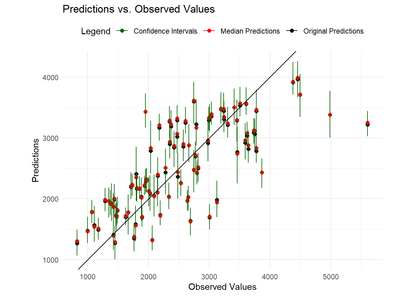
We can see that the original predictions (means) and medians are closely aligned.The predictions generally seem to follow the line at lower values and with shorter Confidence Intervals. This suggests that the model has reasonable predictive accuracy at lower values. However, at higher values of the observed data, some predictions are away from the line with wider confidence intervals indicating higher uncertainty of the predicted values.
Part 3
Now doing a final evaluation of the model with all the predictors. In this case I will use the fitted model to make predictions on the test data test_data3.
#Create a prediction using the test data, for the model with all the predictors
lmall_predtest <- predict(lm_all, new_data = test_data3)

#Match predicted with observed
lmall_predtest <- bind_cols(lmall_predtest, test_data3)

#Estimate the metrics for the model with all the variables as predictors
lmall_metrictest <- metric_set(rmse) #Set the function
lmall_metrictest(lmall_predtest, truth = Y, estimate = .pred) #Compute the RMSE
# A tibble: 1 × 3
.metric .estimator .estimate
<chr> <chr> <dbl>
1 rmse standard 518.And then, plotting the observed vs predicted values of this model
#EDIT THIS PART
#Plotting of predicted vs observed data
ggplot(lmall_predtest, aes(x= Y, y= .pred))+
  geom_point(aes(y = .pred), color = "orangered2", size= 3)+
  geom_point(aes(y = Y), color = "steelblue2", size= 3)+
  geom_abline(intercept = 0, slope = 1, linetype = "dashed", color = "gray20")+ #Draw the 45 degree line
  xlim(0, 5000)+ #Set the x limits
  ylim(0, 5000)+ #Set the y limits
  labs(x= "Observed values", y= "Predicted values")+
  theme_classic()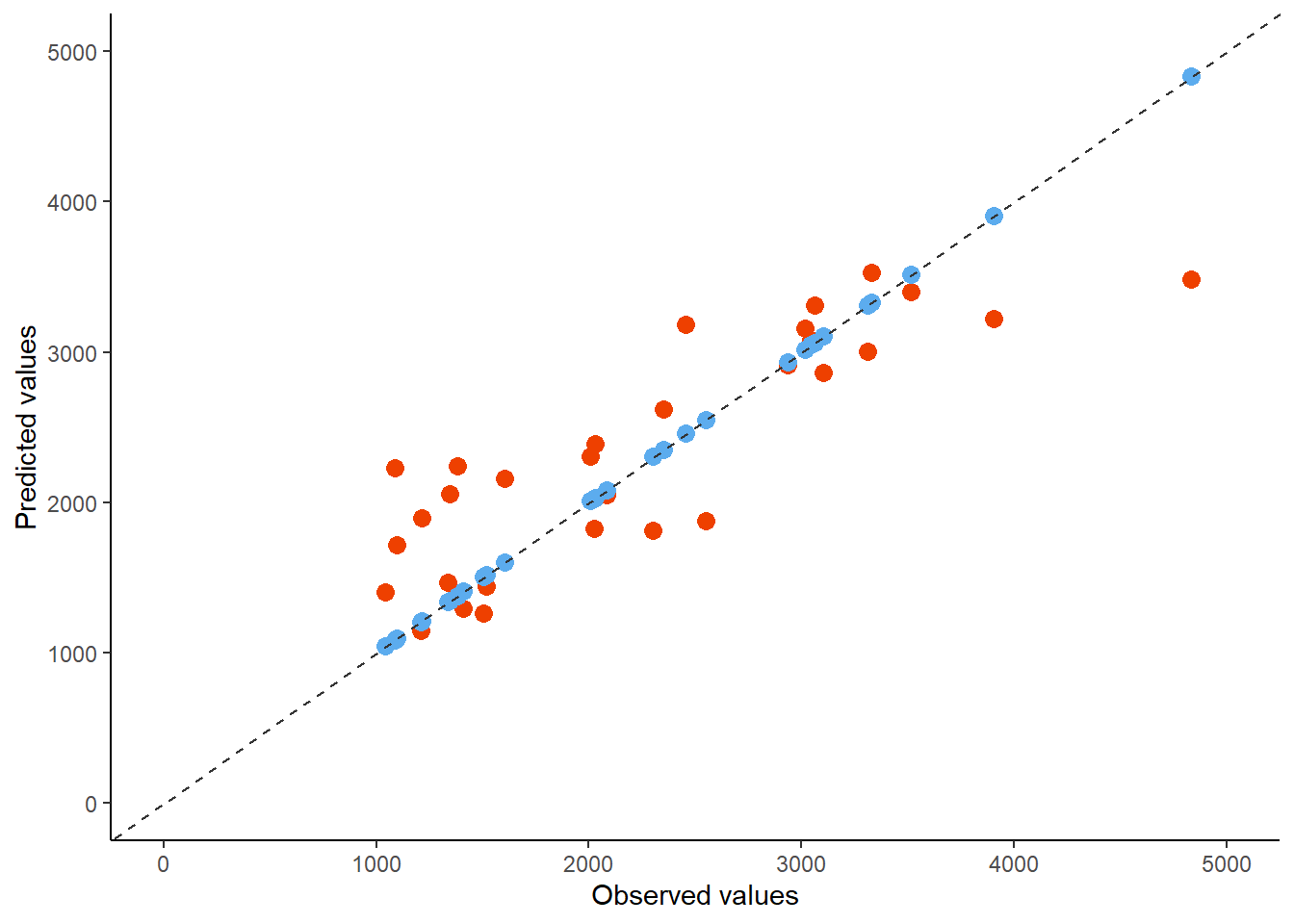
Overall Model Assessment
In general, the model with all the variables as predictors (Model 2) seems like the better fit compared to the model where it was used only Dose as a predictor. A good starting point was comparing the RMSE metric between both models and including a null model as reference. In this case, the null model performed the least, which was expected, and Model 2 perfomed better. The next part, which was to conduct an assessment using cross-validation was another way to assess for the validity of the model. Even though in this case we only assessed Model 2 with CV, it was observed that the uncertainties were relatively small when conducting bootstrap. Finally, the next part was to fit the model with a data set split for testing (test data), and it was observed that the predicted values follow a similar patters as observed from the observed values.
In this case, we chose the most appropriate model in a manner that it doesn’t overfit the data. However, I believe a most accurate model could have been estimated if we had collected other variables. There might be stronger predictors that also, could be generalized to a larger population. I also believe that other metrics such as MAE or R2 could be added to the model assessment so they help in the model selection process.