Registered S3 method overwritten by 'GGally':
  method from
  +.gg   ggplot2
library(glmnet)
Loading required package: Matrix
Attaching package: 'Matrix'
The following objects are masked from 'package:tidyr':

    expand, pack, unpack
Loaded glmnet 4.1-8
library(ranger)
Warning: package 'ranger' was built under R version 4.3.3
Feature engineering
Load the .RDS file and assign it to the mavoglurant dataframe. But first, set a random seed.
#Set the seed to rngseedrngseed =1234set.seed(rngseed)#Load the dataframemavoglurant <-read_rds(here("ml-models-exercise", "mavoglurant.RDS"))
Process the variable RACE, so the values 7 and 88 are encoded as 3.
#Mutate 7 and 88 to 3, for the variable `RACE`.mavoglurant <- mavoglurant %>%mutate(RACE =ifelse(RACE %in%c(7, 88), 3, RACE))
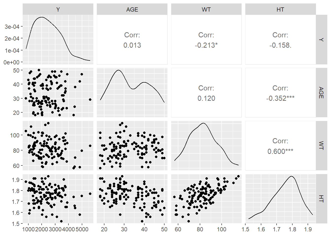
Creating a correlation plot for the continuous variables: Y, AGE, WT and HT
#Creating a correlation plot using the ggpairs() function from the GGally package.ggpairs(mavoglurant, columns =c(1, 3, 6, 7), progress = F)
Seems like there is not much correlation between the variables, except with Height and Weight (R-square: 0.60). Based on this, I created the variable BMI.
Now, creating a new variable BMI, using HT and WT.
#Create the variable BMI, which is computed by dividing the weight (kg) between height-squared (meters)mavoglurant <- mavoglurant %>%mutate(BMI = WT / HT^2)
Model building
First, creating the recipe that will work for all the models
# Create a recipe for preprocessingrecipe <-recipe(Y ~ ., data = mavoglurant) %>%step_dummy(all_nominal(), -all_outcomes()) %>%step_zv(all_predictors()) %>%step_normalize(all_predictors())
Linear Model
Now, setting the specifications for the linear model that considers all the variables as predictors of Y.
#Set seed for reproducibilityset.seed(rngseed)#Define the linear model specificationslinear_spec <-linear_reg() %>%set_engine("lm") %>%set_mode("regression")#Fit the linear modellinear_fit <-workflow() %>%add_recipe(recipe) %>%add_model(linear_spec) %>%fit(data = mavoglurant)
LASSO Model
Here, the specifications for the linear model using LASSO. Using a penalty of 0.1.
#Set seed for reproducibilityset.seed(rngseed)#Define the LASSO model specificationslasso_spec <-linear_reg(penalty =0.1, mixture =1) %>%set_engine("glmnet") %>%set_mode("regression")#Fit the LASSO modellasso_fit <-workflow() %>%add_recipe(recipe) %>%add_model(lasso_spec) %>%fit(data = mavoglurant)
Random forest model
And the specifications of the Random forest model.
#Set seed for reproducibilityset.seed(rngseed)#Define the random forest model specificationsrf_spec <-rand_forest() %>%set_engine("ranger", seed = rngseed) %>%set_mode("regression")#Fit the Random forest modelrf_fit <-workflow() %>%add_recipe(recipe) %>%add_model(rf_spec) %>%fit(data = mavoglurant)
Model performance
First, making predictions for each model and then estimating the RMSE.
#Set seed for reproducibilityset.seed(rngseed)#Compute the predictionslinear_preds <-predict(linear_fit, new_data = mavoglurant) #Linear model with all variableslasso_preds <-predict(lasso_fit, new_data = mavoglurant) #LASSO modelrf_preds <-predict(rf_fit, new_data = mavoglurant) #Random forest model#Match predicted values with the observed for each modellinear_preds <-bind_cols(linear_preds, mavoglurant) #Linearlasso_preds <-bind_cols(lasso_preds, mavoglurant) #LASSOrf_preds <-bind_cols(rf_preds, mavoglurant) #Random forest#Compute the RMSE for each modellinear_rmse <-linear_preds %>%rmse(truth = Y, .pred)lasso_rmse <- lasso_preds %>%rmse(truth = Y, .pred)rf_rmse <- rf_preds %>%rmse(truth = Y, .pred)#Print RMSEsprint(paste("Linear Model RMSE", linear_rmse))
[1] "Linear Model RMSE rmse"             "Linear Model RMSE standard"
[3] "Linear Model RMSE 580.404162763224"
print(paste("LASSO Model", lasso_rmse))
[1] "LASSO Model rmse"             "LASSO Model standard"
[3] "LASSO Model 580.455633646925"
print(paste("Random Forest Model", rf_rmse))
[1] "Random Forest Model rmse"
[2] "Random Forest Model standard"
[3] "Random Forest Model 389.671751733989"
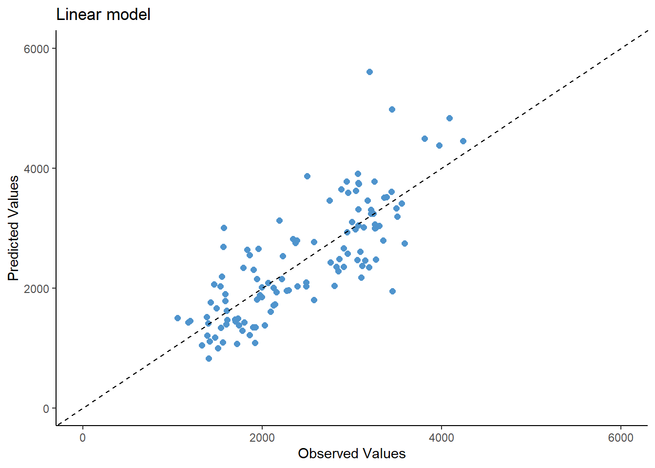
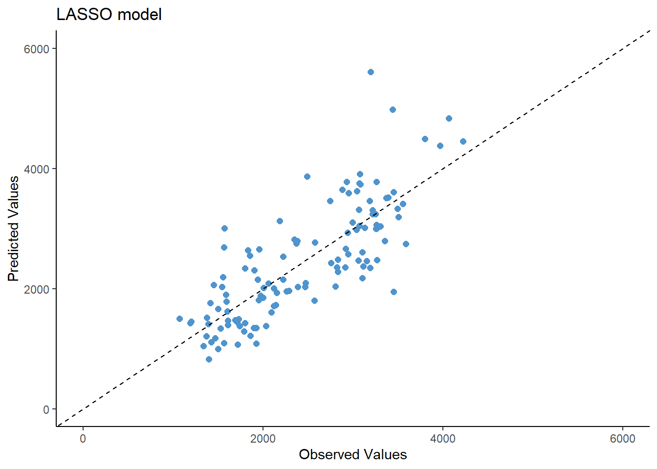
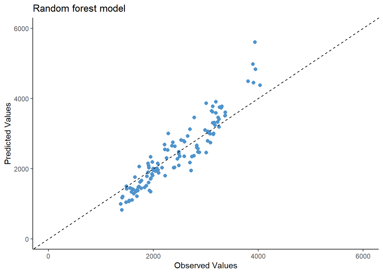
And now, making plots of the observed vs predicted values for each model.
As observed in the model evaluation, the RMSE is pretty much similar between the linear regression and LASSO regression models (RMSE= 580) and the observed vs predicted values seems almost the same. This could be due to the low penalty of the lambda parameter (0.1). However, the random forest seems to have a better performance (RMSE= 389) but still, the predicted values fit similar to the observed values.
Tuning the models
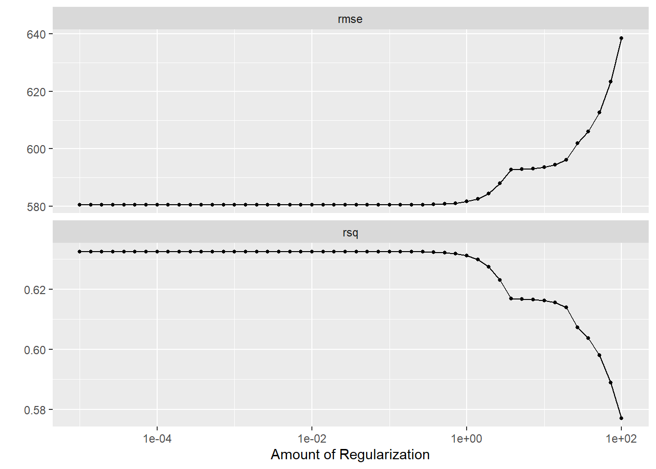
First tuning the LASSO regression model, creating a grid from -5 to 2, every 50 values, and assessing the results using autoplot()
#Define the modellasso_spec2 <-linear_reg(penalty =tune(), mixture =1) %>%set_engine("glmnet") %>%set_mode("regression")#Define the grid of parameterslambda_grid <-grid_regular(penalty(range =c(-5, 2)), levels =50)#Create resamplesset.seed(rngseed)mavo_resample <-apparent(mavoglurant)#Tune the LASSO modellasso_tune_results <-tune_grid( lasso_spec2, recipe, resamples = mavo_resample, grid = lambda_grid)#Diagnostics with autoplotlasso_tune_results %>%autoplot()
It is observed that the RMSE is lower at lower penalization parameters, and the R-squared value is also higher at those lower parameters. It is also seen that the lowest RMSE is similar to the RMSE from the original linear model (RMSE= 580), since the lower tuning does a penalty that mimics dropping a predictor, very similar to the linear model, so the models are pretty much similar.
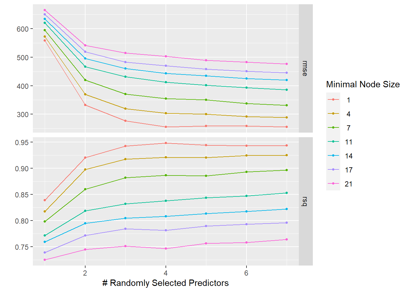
Now the tuning of the Random forest model, creating a grid that tunes the parameters mtry from 1 to 7 and min_n from 1 to 21 every 7 values. Then observing the results using autoplot().
# Define the model for Random Forestrf_spec2 <-rand_forest(trees =300,mtry =tune(), #tuning the mtry parametermin_n =tune()) %>%#tuning the min_n parameterset_mode("regression") %>%set_engine("ranger", seed= rngseed)# Set up the tuning gridtune_grid <-grid_regular(mtry(range =c(1, 7)), min_n(range =c(1, 21)), levels =7)# Perform the tuning for the RF modelset.seed(rngseed)rf_tune_results <-tune_grid(object = rf_spec2,preprocessor = recipe,resamples = mavo_resample,grid = tune_grid)# Plot the resultsrf_tune_results %>%autoplot()
It is observed that for this model, the lowest value of min_n leads to the best model results (RMSE ~ 250, R-squared ~ 0.94).
Tuning with Cross-validation
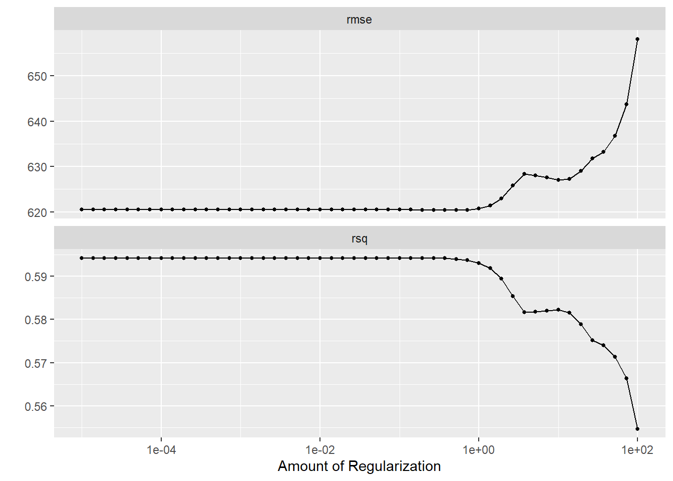
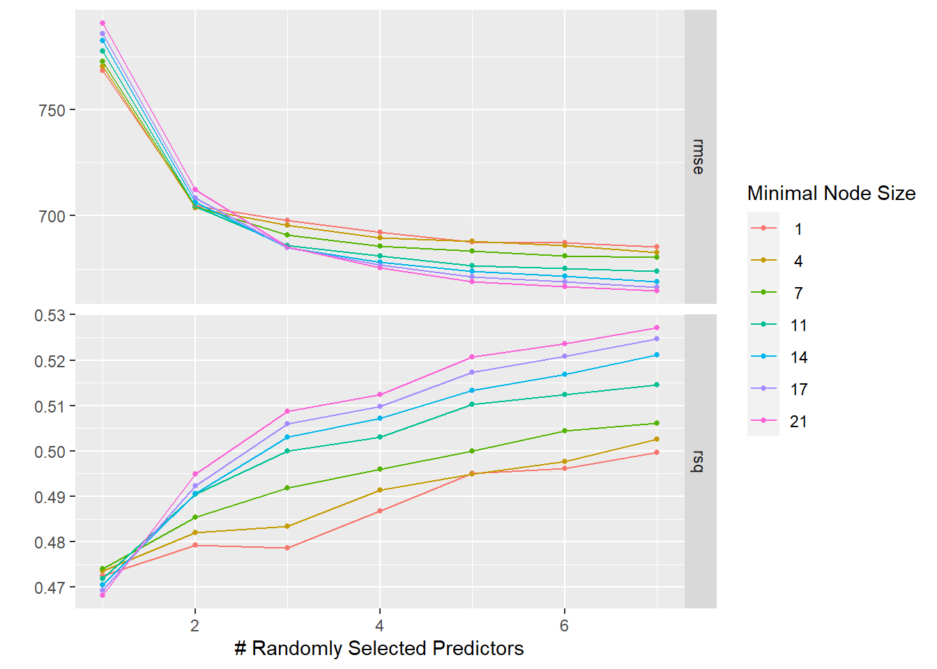
This time, instead of creating resamples with apparent(), I created resamples using cross-validation. The rules are: 5-fold cross-validation and 5 times repeated. Then, tuning both the LASSO and Random forest models with the resamples created.
# Create resamples using cross-validation, and re-setting the seedset.seed(2302)mavo_resample2 <-vfold_cv(mavoglurant, v=5, repeats =5)#LASSO# Tune the LASSO modellasso_tune_results2 <-tune_grid( lasso_spec2, recipe, resamples = mavo_resample2, grid = lambda_grid)# Diagnostics with autoplotlasso_tune_results2 %>%autoplot()
#RANDOM FOREST# Perform the tuning for the RF modelset.seed(2302)rf_tune_results2 <-tune_grid(object = rf_spec2,preprocessor = recipe,resamples = mavo_resample2,grid = tune_grid)# Plot the resultsrf_tune_results2 %>%autoplot()
It is observed that for both models, the RMSE increased. This is due to the re-sampling technique used, this time doing an actual re-sampling using cross-validation. The lowest tuning still seems better for the LASSO model, which is similar to what we observed from the linear regression model. For the Random forest model, the highest min_n parameter approaches to the best model since the lowest RMSE is observed and the highest R-square value. The random forest in this case will provide the best model, but at the cost of overfitting. Meanwhile the linear or the LASSO regression model provide a good model that will perform well on different data to make predictions.